Goldberg Tarjan Push Relabel Algorithm Technische Universität München

Introduction
Create a graph
Run the algorithm
Description of the algorithm
More

The maximum s-t flow has a value of 6

The maximum flow problem

Suppose that we have a communication network, in which certain pairs of nodes are linked by connections; each connection has a limit to the rate at which data can be sent. Given two nodes on the network, what is the maximum rate at which one can send data to the other, assuming no other pair of nodes are attempting to communicate? (source)

This is a typical instance of a maximum flow problem: given an underlying network, where the edge weights denote the maximum possible capacity per edge, one wants to find out how much can be transerred over the edges from the source node s to the target node t.

This applet presents Goldberg Tarjan's Push Relabel algorithm with the FIFO selection rule which calculates the maximum s-t flow on a directed, weighted graph in \(O(|V|^3)\). This is much faster than the older Edmonds-Karp or Dinic's algorithm, which are based on the Ford-Fulkerson method.

What do you want to do first?

maxflow-graph-editor.svg

Legende

	node
	edge with capacity

Which graph do you want to execute the algorithm on?

Start with an example graphs:

Select

Modify it to your desire:

To create a node, make a double-click in the drawing area.
To create an edge, first click on its start node and then on its end node. Alternatively, you may (single-)click on the drawing field to create a new node as end node.
Right-clicking deletes edges and nodes.

Maxflow specific:

The maximum capacity of an edge can be changed by a double-click on the edge or its weight.

Download the modified graph:

Download

Upload an existing graph:

occured when reading from file:

the contents:

What next?

Graph G maxflow-graph-algorithm-graph.svg

Legende

	source and target nodes
	current node
	active nodes
	edge with flow ≤ cap
	flow in blue, capacity in gray corresponding to thickness

Residual Graph G' with axis: fixed maxflow-graph-algorithm-height.svg

Legende

	Active node with height/excess. The height of the bar corresponds to the excess.
	Residual edges e' with their residual capacities c' leaving the current node. Ineligble edges are gray.
	Residual edge used for push.
	Residual edge to minmum height neighbour used for relabel.

Algorithm status

fast forward

Explanation
Pseudocode
Log

First choose a source node

Click on a node to select it as the source/starting node s

Then choose a target node

Click on a node to select it as the target/sink node t. If you want to change the source node, go back with prev.

Goldberg-Tarjan Push-Relabel maximum flow algorithm

Source and target node have been selected and are filled with green. Per default, these are the nodes with lowest and hightest id. If you want to change the target node, go back with prev.

Edges are annotated with preflow/capacity, where the latter corresponds to the thickness of the gray line.

Now the algorithm can begin. Click on next to start it

Initializing the preflow

Set the preflow f(e) (light blue) to the maximum capacity c(e) for all edges emanating s and set f(e) = 0 for all other edges. Add all nodes v ≠ t having (s,v) ∈ E to the queue Q of active nodes (yellow).

The edges in G are labeled with f(e)/c(e) denoting the current preflow along the edge and its maximum capacity. The nodes in G' are labeled with height/excess, where the latter one is also shown as a bar next to the node.

Initializing the height function

For each node v ≠ s set h(v) to the shortest directed path from v to t in the network G where the length of a path is the number of edges of the path. (In particular, set h(t) = 0). This can be done in time O(|V| + |E|) by a breadth first search starting at t and using all edges in the opposite direction. The source s isn’t reached by this BFS. We initialize h(s) by setting h(s) = |V|.

We mapped the height of a node to the y axis in G'.

Main loop

As long as the queue Q containing the active nodes (in yellow) isn’t empty pop the first node v from the front of the queue. We call v the current node and fill it with red.

In the following, we will try to apply push or relabel operations to v to get rid of its excess flow e(v). These operate on the residual edges E' in G' leaving the active node and are displayed with dashed lines and labeled with their residual capacities c'.

Check for admissible push operations

While the current node has excess e(v)>0 and the residual network G'=(V,E') contains an edge that is eligible or legal with respect to the current height function, i.e. there is an edge e'=(v,w) having h(v)==h(w)+1, we can apply a push operation.

All residual edges which are not legal are grayed out. If there is a legal residual edge e' it is displayed in orange.

Push

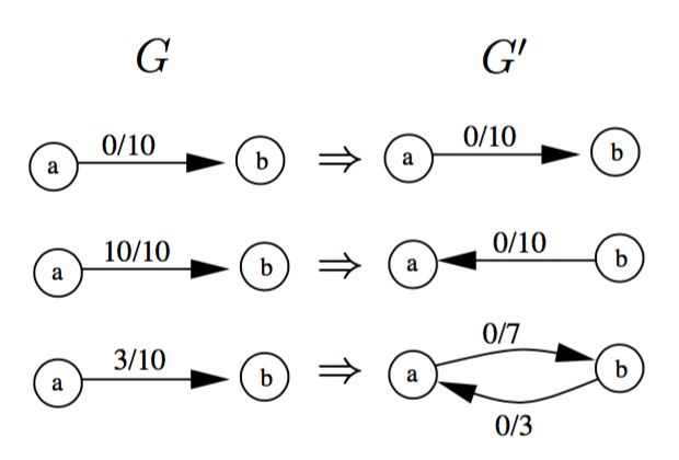
Push δ = min{e(v), c'(e')} amount of flow from v to w. More precisely, if e' ∈ E' is a forward edge (-->) with respect to an edge e of G, increase the preflow f(e) of e by δ, and if e' is a backward edge (<--), then decrease the preflow f(e) of e by δ.

By doing so, e(v) is decreased by δ, and e(w) is increased by δ. If w ≠ s,t, and if w wasn't active before, w becomes active, and is added at the end of the queue Q containing the active nodes.

Check for an admissible relabel operation

If the current node still has excess e(v)>0 and if there is no legal edge emanating from v in the residual network, then apply a relabel operation.

Relabel

Increase the height h(v) of the current node so that it is exactly one level above the minimum height of its adjacent nodes in the residual Graph G'. The residual edge e* to the adjacent node of minimum height is displayed in purple.

Since the current node still has excess, re-add it to the end of the queue Q of active nodes after that.

Finished

The algorithm terminated with a maximum flow value of:

Last operation:

Variable status:

v	Q	e'	e*
-	∅	-	-

s ← pick(v)

t ← pick(v)

BEGIN

(* Initialize the preflow *)

FORALL e=(u,w) ∈ E

f(e) ← (u == s) ? c(e) : 0

IF u == s AND w ≠ t THEN Q.add(w)

(* Initialize the height function *)

h(s) ← |V|

FORALL v ∈ V\{s}

h(v) ← #arcs on shortest v-t path

(* Main Loop *)

WHILE Q ≠ ∅

v ← Q.pop()

WHILE e(v)>0 AND ∃ e'=(v,w)∈E'|h(v)==h(w)+1

(* PUSH *)

push min(e(v),c'(e')) flow from v to w

IF w ≠ s,t AND w ∉ Q THEN Q.add(w)

IF e(v)>0

(* RELABEL *)

h(v) ← 1+min({h(w)|e*=(v,w)∈E'})

Q.add(v)

END

Graph \(G=(V,E)\) with capacities \(c(e)\geq0 \forall e\in E\)

Maximum Flows

In many applications one wants to know how much flow of a certain resource can simultaneously be transferred over a network from a to b. Depending on the context, flow can mean different things: The amount of water in a water pipe system in your city or the bandwidth of a computer network. However, the links in the network on paths from a to b can only handle flow up to their maximum capacity. One now seeks an assignemt of flow values to edges that fulfills all the capacity constraints of the edges and the flow conservation property on all the inner nodes, meaning we don't want leaks in our pipe system.

In general we speak of a flow. Therefore one assigns a flow value to each edge in our network, the graph

The Push-Relabel Algorithm of Goldberg and Tarjan computes the maximum s-t flow on a graph

Flow in graphs

digraph \(G = (V, E)\)

A flow network \( N=(G,c,s,t) \)

capacity \(\forall e \in E: c(e) \geq 0 \)
source and sink \( s,t \in V \)

A flow on N: \( f : E \rightarrow \mathbb{R}_o^+ \)

feasability / capacity constraints: \( \forall e \in E : f(e) \leq c(e) \)
flow conservation: \( \forall u \in V \setminus \{s,t\} : \sum_{v \in V} f(u,v) = \sum_{v \in V} f(v,u)\)

flow conservation: \( \forall u \in V \setminus\{s,t\}: e(u) = 0\)

The residual network

create the residual network

For a (not necessarily feasible) flow \(f : E \rightarrow \mathbb{R}\) in \(G = (V,E) \) we can construct the so called residual network \(G' = (V, E') \): Create the graph G0 from G by copying all nodes of G and adding edges to G0 under the following rules.

Idea of the algorithm

preflow

preflow: \( \forall u \in V \setminus\{s,t\}: e(u) \geq 0\)

height function

height \( h(u), u \in V \)

excess

exess \( e(u) = \sum_{v \in V} f(u,v) - \sum_{v \in V} f(v,u), u \in V \)

What is the pseudocode of the algorithm?


Input:  a directed graph G=(V,E) with source node s, target node t.
        edge capacities c(e)>=0 for all edges
Output: A feasible maximum s-t flow f(e) satisfying:
        capacity constraints : 0<=f(e)<=c(e) for all edges
        flow conservation : f(u,v) == f(v,u) for all nodes except s,t
        The flow value of f(e) is maximized along all feasible flows

How fast is the algorithm?

The running time of the generic Goldberg and Tarjan's push relabel algorithm (1988) is \( O(|V|^2|E|) \).

This is the same asymptotical performance as that of Dinic's algorithm (1970), itself a tuned version of Edmonds–Karp algorithm \( O(|V||E|^2) \). These two classical maximum flow algorithms, emerging from the Ford-Fulkerson method (1956) are based on augmenting s-t paths and preserve the flow conservation property at inner nodes (e.g no excess) even during the course of the algorithm.

So why did we even need another method if it is not asymptotically faster than the existing ones and adds additional complexity? It turns out that we can further tune the generic algorithm by specifiing the order in which we choose the active nodes which we apply push and relabel operations to.

In particular, the variant implemented in this applet chooses the FIFO rule when selecting active nodes from the queue Q, which has a running time of \( O(|V|^3) \), which is better than the previous bound, especially on dense graphs (it is actually independend on the number of edges).

Certain modifications of the generic algorithm are among the fastest algorithms known today to solve maximum flow problems. For a comparison, please refer to this table.

When does the algorithm terminate?

The algorithm terminates when the queue containing the active nodes is empty. When that happens, the preflow is also a feasible maximum flow since the residual network doesn’t contain augmenting pathes from s to t (since d(s) = |V|).

Goldberg and Tarjan about the History of Efficient Maximum Flow Algorithms algorithms (video)

Efficient Maximum Flow Algorithms from CACM on Vimeo.

source: [GT2014]

References

Literature

[GT88] (primary)

Andrew V. Goldberg und Robert E. Tarjan. „A new approach to the maximum-flow problem“. In: J. Assoc. Comput. Mach. 35.4 (1988), S. 921–940. issn: 0004-5411. doi: 10.1145/48014.61051. url: http://dx.doi.org/10.1145/48014.61051.

[GT2014]

Andrew V. Goldberg and Robert E. Tarjan. 2014. Efficient maximum flow algorithms. Commun. ACM 57, 8 (August 2014), 82-89. DOI=http://dx.doi.org/10.1145/2628036.

[AMO93]

Ravindra K. Ahuja, Thomas L. Magnanti und James B. Orlin. Network flows. Theory, algorithms, and applications. Prentice Hall, Inc., Englewood Cliffs, NJ, 1993, S. xvi+846. isbn: 0-13-617549-X.

7.6: Generic Preflow-Push Algorithm
7.7: FIFO Preflow-Push Algorithm
7.8: Highest-Label Preflow-Push Algorithm
7.9: Excess Scaling Algorithm

[Jun13]

Dieter Jungnickel. Graphs, networks and algorithms. Fourth. Bd. 5. Algorithms and Com- putation in Mathematics. Springer, Heidelberg, 2013, S. xx+675. isbn: 978-3-642-32277-8; 978-3-642-32278-5. doi: 10.1007/978-3-642-32278-5. url: http://dx.doi.org/10.1007/978-3-642-32278-5.

6.6: The Algorithm of Goldberg and Tarjan

Algorithm 6.6.1 (generic)
Algorithm 6.6.14 (FIFO preflow push algorithm)
Algorithm 6.6.16 (Highest label preflow push algorithm)

[Cor09]

Thomas H. Cormen. Introduction to algorithms. MIT press, 2009.

26: Maximum Flow

26.4: Push-relabel algorithms
26.5: The relabel-to-front algorithm

The maximum flow problem

This applet presents Goldberg Tarjan's Push Relabel algorithm with the FIFO selection rule which calculates the maximum s-t flow on a directed, weighted graph in \(O(|V|^3)\). This is much faster than the older Edmonds-Karp or Dinic's algorithm, which are based on the Ford-Fulkerson method.

What do you want to do first?

Legende

Which graph do you want to execute the algorithm on?

Start with an example graphs:

Modify it to your desire:

Download the modified graph:

Upload an existing graph:

What next?

Legende

Legende

Algorithm status

First choose a source node

Then choose a target node

Goldberg-Tarjan Push-Relabel maximum flow algorithm

Initializing the preflow

Initializing the height function

Main loop

Check for admissible push operations

Push

Check for an admissible relabel operation

Relabel

Finished

Last operation:

Variable status:

Maximum Flows

Flow in graphs

The residual network

Idea of the algorithm

preflow

height function

excess

What is the pseudocode of the algorithm?

How fast is the algorithm?

When does the algorithm terminate?

Goldberg and Tarjan about the History of Efficient Maximum Flow Algorithms algorithms (video)

References

Literature

Web resources